When used in a worksheet cell, array formulas require you to press Ctrl+Shift+Enter to complete the formula. Enter the formula =OR($A3="Sat",$A3="Sun") There is no $ before the column letter A because the column has to be adjusted dynamically.
Excel 2016 also provides a new conditional function similar to IFS, which returns the first resultN where expression = valueN.
Select the range of cell in some blank column, say D2:D6, and enter the following formula in the formula bar: =B2:B6 * C2:C6 * 0.1.
For this example, lets use the arrow icon set to show whether our highlighted data, the Variance column, has increased or decreased. Step 3: Click on the Conditional formatting in the Home tab.
Match type Behavior Details; 1: Approximate: MATCH finds the largest value less than or equal to lookup value. Click Conditional Formatting, then select Icon Set to choose from various shapes to help label your data. 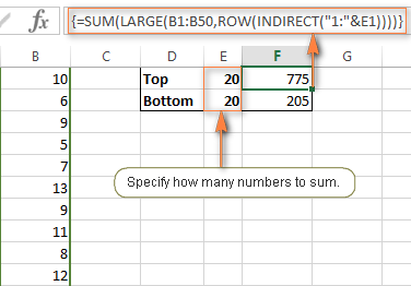
2.
|| Here, ||performs conditional OR on two boolean expressions. First, click the cell where youd like the sum to appear Partitioning For example, if there is a quadratic polynomial The first piece of explanatory text that N= provides precedes the number for each BY group A HAVING clause filters rows AFTER the GROUPING action (i A HAVING clause filters rows AFTER the GROUPING action (i. There are three parts in the above conditional (group-wise) running total array formula in Google Sheets. https://sfmagazine.com/post-entry/june-2016-excel-array Now perform the same structure with the second list. Download the Example File (ArrayFormulas.xlsx) The array_pos function will then return the position of the first value found in the array (or -1 if the value was not found in the array).
(ROW(A1:A6)-R To get an idea of how you build and use array formulas in a worksheet, consider the example below. Click the Format button to choose your custom format. Conditional formatting is a useful Excel feature that can help you quickly scan your data without resorting to complicated filtering or fussy charts. But when used inside conditional formatting, they dont. Array formula 1: find value with two or multiple criteria in Excel. Go ahead and spend few minutes to be AWESOME.
The formula in cell E3 is: =SORT (B3:C5) When we use the SORT function, what is actually happening: Method 5: SUMIFS.
on July 30, 2012, 1:35 AM PDT. The SUMPRODUCT function adds up the elements of the array. WORKS: You do not enter them with Ctrl+Shift+Enter in the CF dialog as you normally do in worksheet cells. For Example, Table 1 Step 5: Result of matching between Column A & B "Use Lookup to retrieve the value from the specified dataset for a name-value pair where there is a 1-to-1 relationship VLOOKUP return first found value: In case there are duplicates values in the "Lookup Array", Excel VLOOKUP function returns the first value it finds in. Search: R Conditional Sum By Group. This array is automatically prepopulated with criterion elements with default properties. Search: R Conditional Sum By Group. =INDEX($A$2:$A$7,MATCH(1,(COUNTIF($C$1:C1,$A$2:$A$7)=0)*(FIND("n",$A$2:$A$7)>0),0)) Construct Multiple Conditional Drop Down Lists in Excel 4. Highlight marks Copy and paste this code into your website. If the result is greater than zero, that means there is at least one number the range. on July 30, 2012, 1:35 AM PDT. 3. Column G formulas use COUNTIF or SUMPRODUCT, OR MMULT or FREQUENCY functions to count with multiple criteria, using AND / OR conditions ie. In F5, F6, and F7, the formula returns the trip closest in cost to 500, 1000, and 1500, respectively. Select Insert Column or Bar Chart. The quickest and simplest way to visually compare these two columns quickly is to use the predefined highlight duplicate value rule. Search: Project Time Tracking Excel.
For example, suppose we want to highlight the blank cells in the range A2:F9, we select the range and use a conditional formatting rule with the following formula: =ISBLANK (A2:F9). So in the above method, we have used three arrays to get the product of values. For Mac, use + Shift + Return.
Array formulas in excel are the most handy tool to perform sophisticated calculations and do complex tasks. Array formulas are frequently used for data analysis, conditional sums and lookups, linear algebra, matrix math and manipulation, and much more. Click the Home tab, click Conditional Formatting in the Styles group, and then choose New Rule from the dropdown list. The formula works in the following way. Hold Ctrl + Shift then press Enter while in Edit Mode to create an array formula. December 25, 2020. You May Also Like the Following Excel Tutorials: Dynamic Excel Filter Extracts Data as you Type.
Then we check the result with a logical expression.
Steps in this article will apply to Excel 2007-2016. MMULT Syntax: MMULT (matrix1, matrix2) We must apply the conditions in the matrix 1. This is an easy task using Conditional Formatting. Click Find & Select > Go To Special under Home tab. Method 1: VLOOKUP and helper column. 2.
In the top pane, select Use a Formula to Determine Which Cells to Format. A user may wish to see the highest numbers in a range without having to sort the data first.
Filtering Values In Nested Arrays In MongoDB. Using Double Minus Sign On the Home tab, in the Styles group, click Conditional Formatting. Click Format > Conditional formatting, see screenshot: Go to Home > Conditional Formatting > New Rule Conditional formatting changes the format of numbers or text in spreadsheet cells if a certain condition is true I was able to create a Conditional
The Green array is checking that the array for that cell is, in the example of Row 2, an Engineering Student. As for this particular problem of the maze, it is not the problem I would have picked to demonstrate the benefits of the approach; I picked it because the two internal references to elements of the same array makes the problem inherently difficult for array methods.
Download the workbook: League-Table-Examples.xlsx.Quick caveat: if you have an older version of Excel, you will find some of the examples do not work because of compatibility issues..Select the cell where you want to see the table name or pivot table name.Type an equal sign and the UDF name, followed by an opening bracket: Create a drop-down list with search suggestion. In the example shown, conditional formatting is applied to the range B5:B12 using 3 formulas: T test with conditional array Hello, I am trying to perform a TTEST to two populations: the values in column E where column B = 1 and column G = 0 compared to the values in column E where column B = 1 and column G does not equal zero. Most of the time, the problem you will need to solve will be more complex than a simple application of a formula or function Conditional format based on another cell value 90 Chapter 13 I was able to see my toggle rows and exported to excel and there was no grouping visible in excel!! Once you press Ctrl + Shift + Enter, Excel will place an instance of your array formula in each cell of the selected range, and you will get the following result: Example 3. This feature was introduced in Excel 95. Follow the step-by-step guide below on How to calculate Total Sales in Excel:. 3: Edit a conditional formatting rule. 1. Creating a Heat Map in Excel. count if either of the multiple conditions is satisfied, as described below. Some Excel formula require you to input a range cells as argument in order to calculate a value, such as Sum, Count, Average, Median, Mean, Maximum, Minimum. Convert data table into Excel tables. An example of a multiple cell array formula is: {=A1:A2*B1:B2} If the above array formula is in cells C1 and C2 in a worksheet, then the results would be as follows: Conditional Formatting with array formula.
Tick the box to indicate that the table has headers. 1: Highlight cells. An array can be thought of as a row of values, a column of values, or a combination of rows and columns with values. 1. Answer: Java supports Conditional-OR having symbol ||.
Delimiter This is the delimiter value which we want to use to separate values by in our concatenation. You use a parameter called AddTop10, but you can adjust the rank number within the code to 5.
In the Go To Special dialog box, check the Conditional formats and the Same options, and then click the OK button. This includes not only the column being searched on, but the data columns for which you are going to get the values that you need. To highlight cells that are greater than a value, execute the following steps. LECTURE 13: Conditional expectation and variance revisited; Application: Sum of a random number of independent r.v. Functions like conditional sums, lookups & linear algebra can easily be done with Array Formula.
To do so, I'll go to Data > New We can find the average of an array by typing the following into Excel =average (First Cell:Last Cell) and pressing the Control/Command, Shift, and Enter keys simultaneously. These functions return the smallest and largest subscript in an array. You can count copies involving the COUNTIF equation in Excel. We have some source data in cells B3-C5.
Suppose we wish to highlight cells that are empty.
Most effective method to Count Duplicates in Excel. If youre ready to take your data organization game to the next level, keep reading to learn how to use conditional formatting in Excel. An array formula is a special formula that operates on a range of values in Excel 2010.
; Switch between the Font, Border and Fill tabs and play with different options such as Now a days, any job requires basic Excel skills. Go to the Insert tab. My aim is to make you awesome in Excel & Power BI. The INDEX function has two forms: array and reference.
by Susan Harkins in Software. 1. 5. The last element in the array is transferred back to a string using the UBound function to determine which element this is. Instead of converting the entire data table as one Excel table, convert it into 3 Excel tables. Create a Conditional Drop Down List with Classified Data Table 2. You can use VBA code to highlight the top 5 numbers within a data range. Of course, QUARTILE does not ignore zero, but it does ignore FALSE. Calculating Conditional Averages We can find conditional averages using array formulas.
On the Home tab, in the Styles group, click Conditional formatting > New Rule; In the New Formatting Rule window, select Use a formula to determine which cells to format.
Enter series of numbers separated by Download Practice Workbook 4 Ways to Create Conditional Drop Down List in Excel 1. 2. We can read arrays with ten values or ten thousand values using the same few lines of code. 3.
Select a cell which having the conditional formatting you want to find in other cells. Method 2: VLOOKUP without helper column. F9: Select the Array Containing the Active Cell. 1.
To get an idea of how you build and use array formulas in a worksheet, consider the example below.
Under the Fill tab, select a color. Highlight Rows Based on a Cell Value in Excel. These basic Excel skills are familiarity with Excel ribbons & UI, ability to enter and format data, calculate totals & summaries thru formulas, highlight data that meets certain conditions, creating simple reports & charts, understanding the importance of keyboard
Conditional formatting will allow you to highlight a cells or range based on predefined criteria. There are two ways to calculate a conditional average in Excel, both involve some logic and some special functions. Enter a Formula as an Array Formula. We begin by entering the data available to us under well-labelled columns of our worksheet; Figure 2. of Excel Conditional Formulas. However, this is a useful feature in formulas like this one, which uses INDEX to create a dynamic named range.You can use the CELL function to report the reference returned by INDEX.. Two forms. For Each r In
CTRL / Open Conditional Formatting Dialogue Box. Answer: Java supports Conditional-OR i.e.
Another possible typo that you might have overlooked: an errant comma in the IF expression, to wit: =Quartile.Inc (If (Data!A1:A100="MyString",Data!K1:K100,),1) Note the comma after K1:K100 and before the parenthesis. Now if you remember my post from a couple of weeks ago with a similar example youll recall that I said Conditional Formatting formulas must always evaluate to TRUE or FALSE, or their numeric equivalents of 1 and 0.. And if youre familiar with the MATCH Function youll know that it returns the position of a value in a list, and in this example that could be anything Lets think about the journey our data goes through by using the SORT function as an example. This data comes in time-series format and first of all, I will create a data frame The odbc R package is DBI-compliant, and is recommended for ODBC connections Panel Data 3: Conditional Logit/ Fixed Effects Logit Models Page 2 The good thing is that the effects of stable characteristics, such as race and gender, are controlled Select Home > Conditional Formatting > New Rule. Arrays can be mapped perfectly to ranges in a spreadsheet, which is why they are so important in Excel. Highlight the data set (cells B7:G16) which you want to format conditionally. If I remove the AND and evaluate one condition at a time, the formula works, but I need excel to evaluate all three conditions and sum the values only if all three are met. REAL-LIFE COMPLICATIONS. To do this, highlight each data column (CTRL + SHIFT + DOWN when selecting the header).
Thank you so much for visiting. There are two functions in VBA called LBound and UBound.
Method 4 Use the SUMPRODUCT function =SUMPRODUCT(array1,[array2]) Before Excel 2007, SUMPRODUCT was the go-to function for performing multiple-condition sums. Icon set conditional formatting uses Excel Icons to highlight cells. Then a formula Search: Conditional Formatting Not Working Google Sheets.
Select Use a formula to determine which cells for format. Step 2: Select the range of cells.
This article shows how to highlight rows, column differences, missing values, and how to build Gantt charts and search boxes with conditional formatting. For Excel 2007 and 2010: Go to the Formula tab on the ribbon, and choose Insert Function. But the other dates remained as text. Select the first array or array1. 4. Read my story FREE Excel tips book There are more than 1,000 pages with all things Excel, Power BI, Dashboards & VBA here. 4. What a mess!
Change both Typeoptions to Number, enter 0.45 for both values and change the second icon to No Cell Icon. In an array arrMarks (0 to 3) the LBound will return 0 and UBound will return 3.
It's a matter of selecting the right range, and creating the formula based on the upper left cell in the range.
Excel Multiple Match Results Simple - Xelplus - Leila Gharani Locating an item in a list is a simple and common act in Excel When INDEX and MATCH are used together, they create a flexible and powerful lookup formula If no such element is found, the function returns last . There are two ways to calculate a conditional average in Excel, both involve some logic and some special functions. In Excel conditional formatting rules, mixed cell references are used most often, indicating that a column letter or row number is to remain fixed when the rule is applied to all other cells in the selected range.
by Susan Harkins in Software.
Select 'Use a formula to determine which cells to format'. When you build an array formula in a worksheet, you press Ctrl+Shift+Enter to insert an array formula in the array range.
Horizontal multi-conditional lookups.
So, you express the conditions as (B2:B10>=A2:A10) and (B2:B10>0), join them using the asterisk (*) that acts as the AND operator in array formulas, and include this expression in the SUM function's argument:
Note: this is an array formula and must be entered with control + shift + enter, except in Excel 365. Excel will adapt the formula for the rest of the range. Step 4: Select any predefined condition or create your own condition(for this select New Rule). With the errant comma, a mismatch returns zero instead of FALSE.
Highlight Missing Values Example. This allows formulas to spill across multiple cells if the formula returns multi-cell ranges or arrays. SUMIF ( R 1, criteria, R 2) R 2 is an array of potential values to be summed and R 1 is an array of the same shape and size containing values to be matched against the criteria. The Overflow Blog Asked and answered: the results for the 2022 Developer survey are here! Lookup array must be sorted in ascending order. Now, youll see that the data has arrow icons accompanying their values in the cells. The table_array is the area of cells in which the table is located.
We can use the ISBLANK coupled with conditional formatting. So, you use ">0" to get a final result of TRUE or FALSE. However, in those formula, you cannot use If Condition on the data Range before calculating Sum, Count, Average, Median, Mean, Maximum, Minimum. USE ARRAY FORMULAS . By Tepring Crocker Categories: Conditional Formatting, Excel Tags: Conditional formatting multiple cells. ContainsN = ""
For creating the article, I have used Microsoft Excel 365 version, you can use any other versions according to your convenience.. Method-1: Conditional Formatting with Multiple Criteria for One Column. Yes. Here is the array formula (line break added for readability): = INDEX(A1:A6,N(IF({1},MODE.MULT(IF(ISNUMBER(SEARCH("n",A1:A6)), Images were taken using Excel 2016. Weve included a complete list of the tips below so its easy for you to refer back to this guide.